This paper explores whether momentum exists in professional basketball through a novel entropy-based statistical analysis. Based on the 2019–20 NBA season play-by-play dataset, we apply a clumpiness measure to scoring sequences and simulate expected distributions under different assumptions.
1 Introduction
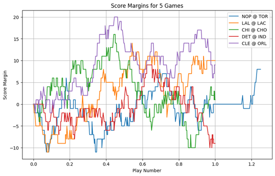
On June 10, 2019, the Toronto Raptors played the Golden State Warriors in Game 5 of the NBA Finals. The Raptors lead the series 3-1 and were looking to raise the Larry O’Brien Championship trophy in front of a home crowd for the first time ever on Canadian soil. The Raptors trailed most of the game, and at the beginning of the fourth quarter, they were down by 6 points. After a back-and-forth exchange of baskets in the first 5 and a half minutes of the quarter, the Raptors click into gear. Kawhi Leonard scored 4 straight baskets interrupted only once by a Draymond two-pointer to take a 6 point lead, the Raptors’ first lead since the first quarter. With 3:28 left on the clock, all of Canada can taste its first championship. After a missed three-point attempt by Steph Curry, the Raptors regain possession with 3:12 to go. Suddenly, with the ball in Kawhi’s hands, the unthinkable: Raptors’ floor general Kyle Lowry calls a full timeout. Fans and pundits alike groan. You simply don’t call a timeout when you are hot. When the Raptors return to the floor, the energy is different. Kawhi misses an 11-footer, Klay drains a three, Lowry misses the retribution three, Curry hits another three, Kawhi misses a three, Klay hits another three, Nurse calls another timeout, presumably to stop the Warriors’ run. The score is now 106-103. When they return to the floor, Lowry scores the Raptors’ final basket of the game a goaltended layup. The Warriors survive game 5. “Basketball is a game of runs”. Those familiar with the sport will have heard this before, and not just from fans, but coaches and announcers. The truth of the statement has been a matter of academic discourse since at least 1985, when Thomas Gilovich, Robert Vallone and Amos Tversky published the first evidence for the opposition. In the 4 decades since, many academics have chimed in with their own evidence for and against. The majority of the literature has been in opposition to statistical momentum, and in fact the rules are specifically designed to increase parity. For instance, all of soccer, American football and basketball award possession of the ball to the team which has just allowed a score, in a process commonly known as “loser’s ball”. Given that ball possession is generally required to score in these sports, preventing a dominant team from immediately capitalizing on their success should make it harder for teams to score consecutively and hence gain momentum. Yet the sentiment of the opening paragraph prevails time and again. Why? Analyzing the score margins for a few games, the general game pattern seems to empirically align with this sentiment. Of course, this is not a statistical approach, but it provides a visual intuition for why we as humans so often perceive momentum, despite both the mean reverting nature of the game and the long-standing literature disproving this notion.
This question has resurged in importance as analytics have become more popular in professional sports. The impact of better decision making could be making the game more momentum driven or less; either way, one thing is sure, the basketball of today’s NBA is not the same as that of Gilovich, Vallone, and Tversky’s NBA. This paper employs a somewhat novel entropy measure of team wide momentum to test scoring event runs in the course of the game. Our innovation is a novel approach to bootstrapping the null hypothesis distribution of hyper-parameter values, which is a MLE weighted combination of the traditional frequency method, and a Markovian transition approach we call the Loser’s ball effect.
Note: “Basketball is a game of runs.” — This was the notion we went into the paper convinved of, in essence meaning that teams go on momentum driven runs.
2 Literature Review
The seminal paper on the topic by Thomas Gilovich and Robert Vallone and Amos Tversky titled “The Hot Hand in Basketball: On the Misperception of Random Sequences” has inspired a slew of literature on the subject of momentum in basketball and sports generally. In their paper, Gilovich et al. (1985) explore the common belief of a player’s hot hand in basketball. The belief holds that when a player hits a shot, they are more likely to hit their next shot, and similarly when they miss the cooling effect decreases their probability of scoring the next shot. The paper looks at both the psychology behind the belief, and the statistics of its validity. The authors studied data from 48 games of the 76ers 1980-81 season, looking at consecutive free throw shooting. Gilovich et al. (1985) use conditional probabilities, Wald-Wolfowitz run tests, a test of stationarity, and an analysis on inter-game stability using Lexis ratio, a method from David (1949). Part of the discussion of the paper is that the players themselves believed in the hot hand, and later papers like Reifman (2011) discuss how player and coach behavior may inhibit streaks from occurring. Bocskocsky et al (2014) challenged the assumption of independent shot selection and provide evidence for the hot hand in basketball. Bocskocsky et al (2014) make reference to Gilovich et al. (1985) and their key assumption of independence (emphasis added).
“It may seem unreasonable to compare basketball shooting to coin tossing because a player’s chances of hitting a basket are not the same on every shot. Lay-ups are easier than 3-point field goals and slam dunks have a higher hit rate than turnaround jumpers. Nevertheless, the simple binomial model is equivalent to a more complicated process with the following characteristics: Each player has an ensemble of shots that vary in difficulty (depending, for example, on the distance from the basket and on defensive pressure), and each shot is randomly selected from this ensemble” (Gilovich, Vallone and Tversky, 1985)
Using data from 83,000 shots taken during the 2012-13 season, as well as optical tracking data, the authors provide evidence for the non-independence of a player outperforming their usual percentage (a hot handed player), suggesting that these players tend to shoot from farther away, face tighter defense leading to more difficult shots. They use OLS regression for a model of shot difficulty. The authors use this predictive model to establish a complex heat which is a definition of heat corrected for difficulty. With these corrections for difficulty and complex heat they once again run an OLS regression, and find a positive and significant coefficient, which roughly translates to a 1.2% increase in shooting percentage for a hot player when controlling for shot difficulty. The key discussion in Bocskocsky et al (2014) relies on the importance of accurately defining heat.
“Concluding that the hot hand exists is contingent on defining “hot” correctly. A player who makes three out of his past four layups is not hot, but a player who makes three out of his past four three-point attempts is. In other words, being hot is not about the absolute number of shots a player has previously made, but rather is about how much he has outperformed, conditional on the types of shots he has taken.”
Both papers were focused on individual player performance. This is distinct from team momentum, especially in the context of correcting for shot difficulty, where to increase the difficulty for the individually hot player, given a finite set of defensive resources, the opposing team must decrease the defense difficulty for the not-hot subset. Reifman (2011) discusses this exact challenge, of the difficulty of measuring streakiness in team performance. Arkes and Martinez (2011) use a correlation test to demonstrate positive momentum between wins. The authors correct for strength of opponents, where again the definition of a hot team is defined to mean outperformance above expectation in the past games rather than simply winning the last few games. Steeger et al. (2021) use an entropy model for NHL hockey to suggest that team momentum over the course of a season at a game-by-game granularity does not exist. The entropy model looks at the interarrival time between wins for each team and bootstraps a statistical significance level from a random binomial draw. The advantage of this method is it does not require stationarity, in essence allowing for a team get better (or worse) throughout the season. Steeger et al. (2021) make no corrections for difficulty of opponent, rather the bootstrapped hyperparameter is calculated based on each team’s individual end of season winning percentage. The entropy measure used in Steeger et al. (2021), was developed in Zhang et al. (2013). The intent of that paper was to develop a non-parametric measure for clumpiness in data. Clumpiness is defined as irregular clusters of data together. Part of the motivation of the Zhang et al. (2013) paper was to create a more powerful statistical measure of clumpiness, in response to the measurement used by Gilovich et al. (1985). One of the advantages in our view of the measure developed by Zhang et al. (2013) is the continuity property. Small changes in the timing of an event have limited effects on the measure. This stands in contrast to a Wald-Wolfowitz run tests which focuses on consecutive sequences of data. For our purposes, the continuity process is important, because in our view the difference between an 8-0 run and a 10-2 run is negligible.
3 Methodology
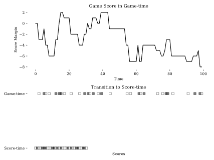
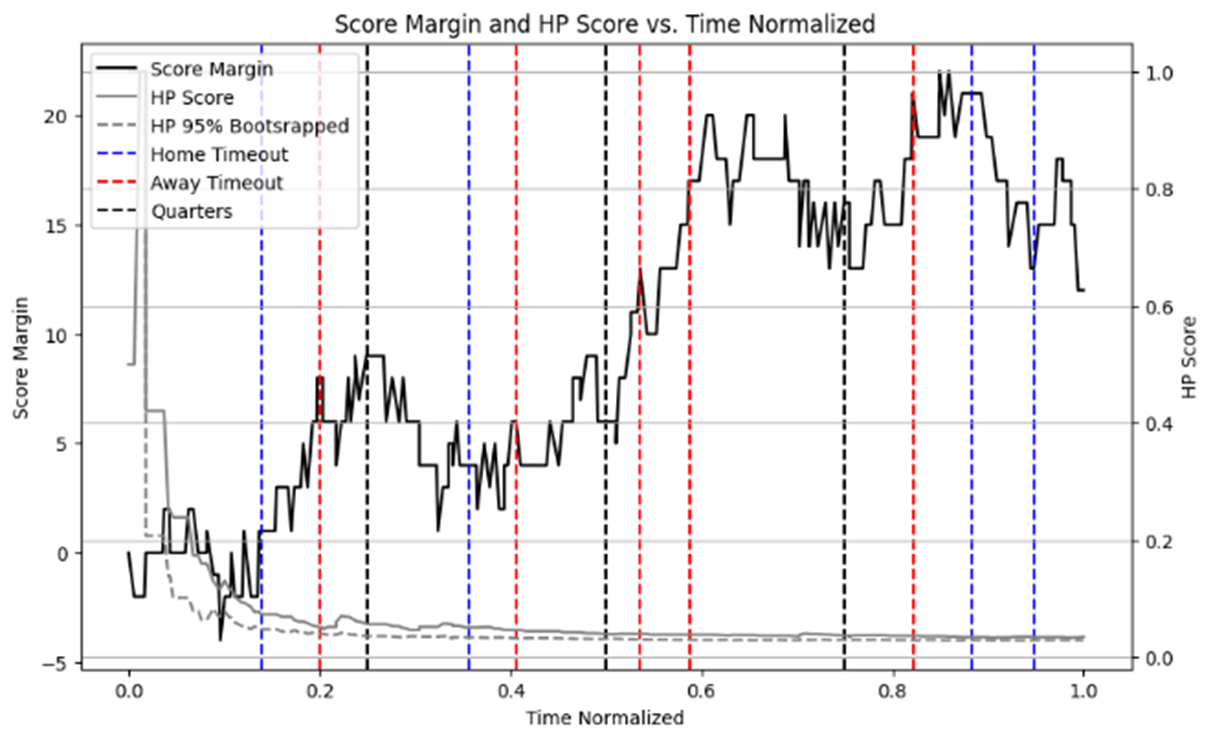
To determine whether scores in a basketball game are clumpier, meaning that a teams points are “clumped” together as they go on and allow runs, than random we use the scaled entropy measure described in Zhang et al. (2014), which is a scaled version of the 2013 measure, due to basketball’s non-fixed number of scoring plays. To calculate entropy we first make two transformations to the data, the first is converting from game-time to what we call score-time. The second is to convert score margin changes into a binary home score variable. Figure 1, gives a visual intuition, which shows the process of first converting score-margin into binary scoring events and then rescaling the time based on number of scoring events.
Let $t$ represent game-time where
\[t \in [0,T]\]And $T$ is the total game duration. Let $H(t)$, $A(t)$ and $S(t)$ be the home score, the away score and the score margin at time $t$ where
\[S(t) = H(t) - A(t)\]We define an indicator function
\[\mathbf{1}_{\Delta S(t)} = \begin{cases} 1, & S(t) \neq S(t - 1) \\ 0, & S(t) = S(t - 1) \end{cases}\]And rescale time to score-time $\tau \in [0,N]$
\[\tau = N(t) = \sum_{i=1}^{t} \mathbf{1}_{\Delta S(i)}\]Such that at game-time T
\[\tau = N(t) = N\]Where $N$ is the total number of scoring events in a game. With this score-time $\tau$ we can determine the inter-event time between home scores. Let $x_i$ be the inter-event time of the $i$th
\[x_i = \begin{cases} \tau_1, & i = 1 \\ \tau_i - \tau_{i-1}, & 2 \leq i \leq n \\ N + 1 - \tau_n, & i = n+1 \end{cases}\]Where $n$ is the total number of home scores and $N$ is still total number of scores. To briefly add intuition, the Toronto Raptors ($A$) played the Philadelphia 76ers ($H$) in Philadelphia on February 11th 2025. The first ten scores of the game went as follows
\[A H A H A A A A A H\]$N$ is 10, $n$ is 3, $x_1$ is 2, $x_2$ is 2, $x_3$ is 6, and $x_4$ is 1. In this sequence the importance of $x_(n+1)$ is not best exemplified. Part of the usefulness of the entropy measure is that its evolution can be tracked throughout a game. Returning to our Raptors game, the first nine scores
\[A H A H A A A A A\]Now $N$ is 9, $n$ is 2, $x_1$ is 2, $x_2$ is 2, $x_3$ is 5. Here we see the $x_(n+1)$ essentially closes the last run.
To standardize across different games, we compute scaled $\tilde{x}_i$
\[\tilde{x}_i = \frac{x_i}{N + 1}\]Such that
\[\sum_{i=1}^{n+1} \tilde{x}_i = 1\]Finally, the normalized entropy (Steeger et al., 2021) is given by
\[H_p = \frac{\sum_{i=1}^{n+1} \tilde{x}_i \log(\tilde{x}_i)}{\log(n + 1)}\]Although higher values indicate more “momentum” and suggesting the alternative, this value remains somewhat meaningless by itself. As such, we bootstrap a p-value at a game level by randomly simulating each game 10,000 times and building the distribution for the testing of the null hypothesis.
In our context, the Steeger et al. (2021) method would use end of game scoring event ratio to simulate each game.
Frequency-based:
\[p_s^g = \frac{S_h^g}{S_h^g + S_a^g}\]Where $S_h^g$ is the number of scoring events in a given game $g$ for the home team $h$ and $S_a^g$ is the number of scoring events for the same game, for the home team $a$. Thus the $p_s^g$ is the probability for a given game that the home team is the scorer of the next scored basket, as in not the next shot, but the next scoring event. It can also be thought of as the relative scoring-event share of the home team for any given game $g$.
An alternative method would account for the “self-balancing” nature of basketball. The rule referred to in basketball as “loser’s ball” essentially means that the team that just allowed a scoring event receives possession of the ball. Other sports, like volleyball, have “winner’s ball”, but these sports tend to have disadvantages associated with possession. The fundamental insight is that professional sports’ rules seem to be designed to increase competition and thereby decrease momentum by facilitating a “back-and-forth” scoring pattern presumably to make the product more entertaining to watch.
In order to bootstrap with this insight, we use a first-order Markov chain, similar to the method used in Albright’s (1993) analysis of hitting streaks. The probability that a given team scores, given the state that they previously score is
Markovian (“loser’s ball”):
\[p_h = P(S_h | H), \quad p_a = P(S_a | A)\]Higher levels of p_h suggest that the home team was better at scoring given they had just scored. Further, if p_h > p_s it would suggest that having previously scored made the home team more likely to score again than their base likelihood of scoring. and…
\[p_AH = 1 - p_h = 1 - P(S_h | H), \quad p_HA = 1 - p_a = 1 - P(S_a | A)\]The transition matrix $M$ is given by
\[M = \begin{bmatrix} p_h & 1 - p_h \\ 1 - p_a & p_a \end{bmatrix}\]Where $P_HH$ is the probability of Home scoring (first $H$) given a previous state of home scored (second $H$). With this transition matrix, we adjust for the self-correcting nature of basketball. It is important to note because we are looking to capture the effect of a rule, we calculate this matrix at a season wide level, though in practice our implementation sums the transitions at a game level to build the season level matrix.
The best bootstrapping method would have a combined probability that considers both the self-correcting nature of basketball, that we call the “losers’ ball” effect, and the overall balance of the individual games scoring events, so that the final scoring event distribution resembles that of the actual game played and isolates the potential differences in process to get to this final result.
To do this, we define $\lambda \in [0,1]$ a weighing factor. Where $\lambda=1$ weights the probability entirely to the games scoring event ratio, and $\lambda=0$ weights the probability entirely to the loser’s ball effect. One important note, where the pure Markov approach was defined by season level parameters only, whereas the incorporation of $\lambda$ leads to a blend of season level parameters and game level variables. Incorporating the weighting factor
\[P_{HH}^g = \lambda p_s^g + (1 - \lambda)p_h\] \[P_{AA}^g = \lambda (1 - p_s^g) + (1 - \lambda)p_a\]The now game level transition matrix $\dot{M}^g$ is given by
\[\dot{M}^g = \begin{bmatrix} P_{HH}^g & P_{HA}^g \\ P_{AH}^g & P_{AA}^g \end{bmatrix} = \begin{bmatrix} \lambda p_s^g + (1 - \lambda)p_h & 1 - \lambda p_s^g + (1 - \lambda)p_h \\ 1 - \lambda (1 - p_s^g) + (1 - \lambda)p_a & \lambda (1 - p_s^g) + (1 - \lambda)p_a \end{bmatrix}\]To better understand the significance of the $\lambda$ parameter, we bootstrapped entropy distributions at different levels of $\lambda$ in increments of $0.1$ based on $p_s \in {0.4,0.5,0.6}$ representing, a bad, average, and good team respectively.
The following figure demonstrates the effect $\lambda$ of on the bootstrapped distribution and resulting statistical significance level.
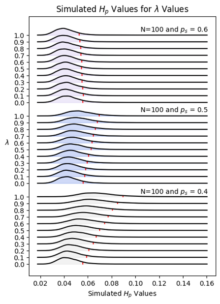
The effect of $\lambda$ at different levels is quite interesting. For good teams, say $p_s=0.6$ the loser’s ball effect decreases the expected amount of entropy. In effect, if a team is better than the loser’s ball effect, then low $\lambda$ values have a dilutive effect. The opposite is true for mediocre and bad teams.
4 Parameter Estimation
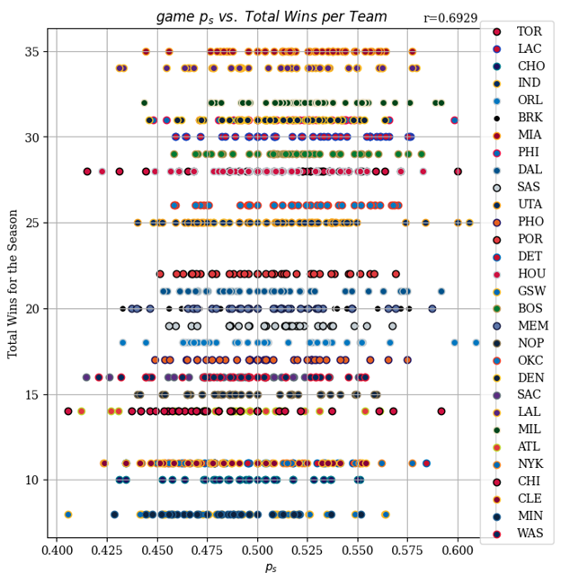
It is clear that both $\lambda$ and $p_s$ are crucial to accurately simulating games for bootstrapped significance levels. To better understand the importance of $p_s$ we plotted each teams game values of $p_s$ and their total home wins in the season. The pearson correlation coefficient was 0.6929. This aligns with our intuition that better teams in general win with a greater share of the scoring events. The width of each teams distribution provides visual intuition for the difficulty of consistent performance in a commodity scoring commodity game league.
$p_s$ is a empirical observation, The level of $\lambda$ clearly makes a meaningful impact on the statistical threshold, and is not observed. Thus it is important that we use a grounded estimate. We used a maximum likelihood estimation approach. We define a log likelihood function of $\lambda$,
\[\ln(L(\lambda)) = \sum_{g=1}^{G} \ln(L_g(\lambda)) = \sum_{g=1}^{G} \left[ N_{HH}^g \ln(P_{HH}^g) + N_{HA}^g \ln(P_{HA}^g) + N_{AH}^g \ln(P_{AH}^g) + N_{AA}^g \ln(P_{AA}^g) \right]\]Finally we optimize for $\lambda^*$
\[\lambda^* = \arg\max_{\lambda} \ln(L(\lambda)) = 0.249\]The estimated value of $\lambda^* $, obtained via maximum likelihood estimation, is $\lambda^*=0.249$ . This suggests that scoring orders are primarily driven by the loser’s ball effect. An important limitation of this finding is that it applies to NBA games. In less competitive leagues we expect the importance of $p_s$ to be significantly higher, but amongst the best players in the world, the relative strength differences of teams is too small to overpower the balancing effect of the loser’s ball rule.
5 Analysis
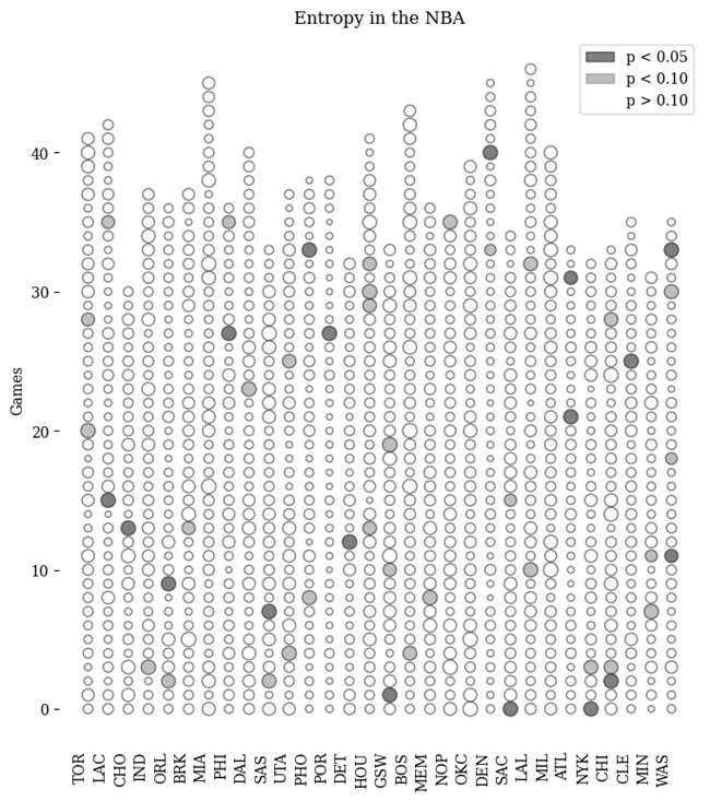
Using entropy as our measure, we considered all games in the 2019-20 season from the home team’s perspective. We find that the majority of games are not statistically significant, but that most teams have somewhere between 1-4 statistically significant games with momentum in a given season. With 1230 total observations, and only 50 statistically significant observations, our primary concern was that we had a multiple compairisons problem.
Our first approach to determining at a season level, whether there is evidence of statistical significance was to bootstrap a seasons worth of entropy values. We can see visually, that there is little differences between the two distributions.

We then compared these distributions using a Mann-Whitney U test.
- U-statistic: 970.0
- P-value: 0.4337 Thus on this measure there is no statistical difference between our hypothesis of momentum in basketball and the null hypothesis of no momentum.
No season-level evidence for momentum exists.
6 Discussion and Results
With the rise of analytics in professional sports and the perseverance of fan misconceptions, we have returned to a classic question at the heart of sports analytics. In this paper, we have explored a novel method for determining data clumpiness. We found 50 of 1230 games with statistically significant momentum. With that many observations, we wanted to avoid a multiple-comparisons problem. Thus, we randomly sampled from the bootstrapped game distribution to bootstrap a season distribution, which we compared to the season’s true distribution. We found no evidence at a season level of statistical difference between our hypothesis of momentum and the null hypothesis of no momentum.
Many areas of further research have piqued our interest in this process. One such area is whether the games that do have statistically significant entropy are experiencing randomness derived entropy or whether, on account of some knowable quantity these games experience momentum derived entropy. Two such ideas present themselves. Whether blowouts are correlated to statistical entropy, and whether timeouts have a dilutive effect to statistical momentum, as the fans and the pundits from our opening paragraph might have you believe.
Further, we can view the changes in entropy and statistical significance at a play by play level (though computationally expensive), which may have managerial implications that might be derived midgame. One such is when to call timeouts.
Another area of exploration would be to compare momentum with different seasons’ datasets to see if and what direction the sport is moving in terms of momentum.
Further Questions
- Are blowouts correlated with statistical entropy?
- Do timeouts affect momentum (as fans often claim)?
- What can be learned midgame from entropy tracking?
Bibliography
Sources
Albright, S. C. (1993). A Statistical Analysis of Hitting Streaks in Baseball. Journal of the American Statistical Association, 88(424), 1175–1183. https://doi.org/10.1080/01621459.1993.10476395
Arkes, J., & Martinez, J. (2011). Finally, Evidence for a Momentum Effect in the NBA. Journal of Quantitative Analysis in Sports, 7(3). https://doi.org/10.2202/1559-0410.1304
Avugos, S., Köppen, J., Czienskowski, U., Raab, M., & Bar-Eli, M. (2013). The “hot hand” reconsidered: A meta-analytic approach. Psychology of Sport and Exercise, 14(1), 21–27. https://doi.org/10.1016/j.psychsport.2012.07.005
Bar-Eli, M., Avugos, S., & Raab, M. (2006). Twenty years of “hot hand” research: Review and critique. Psychology of Sport and Exercise, 7(6), 525–553. https://doi.org/10.1016/j.psychsport.2006.03.001
Bocskocsky, A., Ezekowitz, J., & Stein, C. (2014). Heat Check: New Evidence on the Hot Hand in Basketball. SSRN Electronic Journal. https://doi.org/10.2139/ssrn.2481494
David, F. N. (1949). Probability Theory for Statistical Methods. Legare Street Press.
Gilovich, T., Vallone, R., & Tversky, A. (1985). The hot hand in basketball: On the misperception of random sequences. Cognitive Psychology, 17(3), 295–314. https://doi.org/10.1016/0010-0285(85)90010-6
Reifman, A. (2011). Hot Hand. Potomac Books, Inc.
Schilling, M., 2019, Is basketball a game of runs? arXiv. Retrieved from https://arxiv.org/abs/1903.08716
Steeger, G. M., Dulin, J. L., & Gonzalez, G. O. (2021). Winning and losing streaks in the National Hockey League: are teams experiencing momentum or are games a sequence of random events? Journal of Quantitative Analysis in Sports, 17(3), 155–170. https://doi.org/10.1515/jqas-2020-0077
Wolfowitz. J. (1943). On the Theory of Runs with some Applications to Quality Control. Annals of Mathematical Statistics, 14(3), 280–288. https://doi.org/10.1214/aoms/1177731421
Zhang, Y., Bradlow, E. T., & Small, D. S. (2013). New measures of clumpiness for incidence data. Journal of Applied Statistics 40(11), 2533–2548. https://doi.org/10.1080/02664763.2013.818627